Autoregressive Integrated Moving Average (ARIMA) Models

Introduction

Time series Forecasting is a method to forecast behaviour of future variables on the basis of previously observed variables, based on the underlying assumption that whatever happens in the future is a function of what happened in the past. An approach to handling time-correlated modelling and forecasting is called Autoregressive Integrated Moving Average (ARIMA) models. ARIMA models are popular because they can represent several types of time series, namely: Autoregressive (AR) models, Moving Average (MA) models, combined AR & MA (ARMA) models, and on data that are differenced in order to achieve weak stationarity (I for ‘integrated’). A caveat is that, studies in ARIMA have generally assumed that there exists a linear correlation structure among time series values, therefore complex real-world predictions are not always satisfactory.

Nonetheless, I would like to explore the applications, implementations and performance of ARIMA on the Time Series Analysis of Financial Data. In this project, I will first perform Exploratory Data Analysis on the dataset (Closing prices of S&P 500) to identify Stationarity, Autocorrelation, Partial Autocorrelation, and Order of differencing. Next, I will make predictions with the AR(1) model, MA(1) model, ARIMA(1,1,1) model, ARIMA(1,1,1) out-of-sample forecasts, and then with the SARIMA out-of-sample forecast.

Dataset

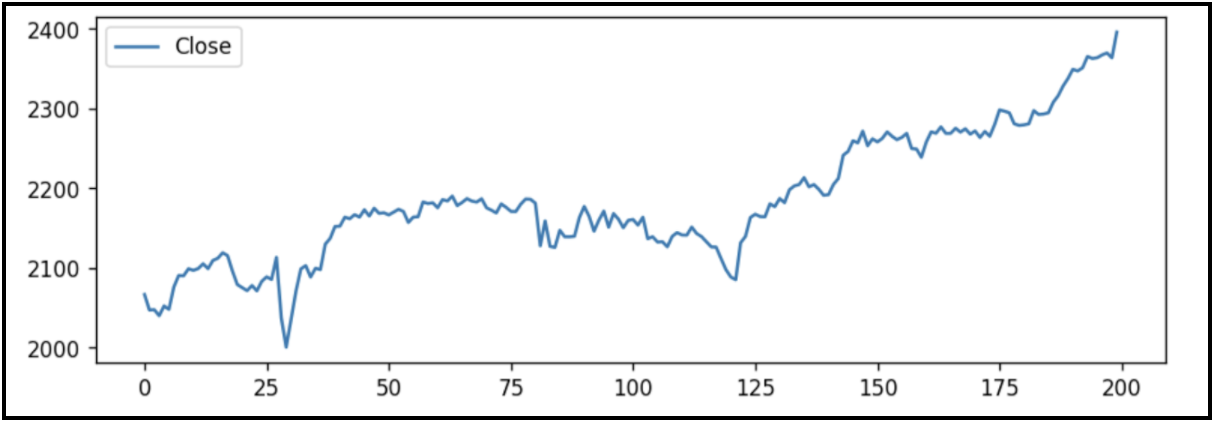
The dataset that I will be using will be the daily closing price of the S&P 500, in the period corresponding to June 2016 – Mar 2017. The reason I chose this time period was because the mean of this period is relatively linear, and it was easier to implement the ARIMA model on linear-mean time periods. I recognise that this would result in biases, but I would like to highlight that the point of the project was to explore the implementations of the ARIMA model and get myself familiar with the ARIMA model.

Exploratory Data Analysis

Stationarity

Stationary processes are processes where its mean, variance and autocovariance do not vary with time. Stationary data are better approximated with time series analysis. We will test whether the S&P 500 data is stationary, with the Augmented Dickey–Fuller (ADF) test implemented by the statsmodels.tsa python package (which we will be using to implement the other models as well).

The null hypothesis of the ADF test is that the time series is non-stationary. So, if the p-value of the test is less than the significance level (0.05), we will reject the null hypothesis and infer that the time series is indeed stationary.

Differencing

Differencing is a method of making a times series dataset stationary, by subtracting the observation in the previous time step from the current observation. This process can be repeated more than once, and the number of times differencing is performed is called the difference order. We can see that a differencing of order 1 is enough to bring the series to a stationary mean but not so much variance. Nonetheless, a differencing order of 1 should be used because first-order differencing addresses linear trends. This means that the order of the “I” term in ARIMA is 1.

Autocorrelation

Autocorrelation is the correlation of a signal with a delayed copy of itself as a function of the time lag between them.

Since we are differencing the dataset only once, we shall look at the autocorrelation of signals for the dataset that is different once. Ideally, we will select a lag that is above the confidence interval. However, there does not appear to have a time lag that is suitable, so we will just select an order of 1. This will contribute to the “q” in the MA(q) term – we will adopt an MA(1) model.

Partial Autocorrelation Function

Partial Autocorrelation Function (PACF) gives the partial correlation of a stationary time series with its own lagged values, regressed the values of the time series at all shorter lags. This means that PACF considers only the direct effect of the lagged values, ignoring all indirect effects of the lagged values.

As before, we will only look at the PACF plot of the 1st order differenced dataset. There does not appear to have a time lag that is suitable, so we will just select an order of 2. This will contribute to the “p” in the AR(p) term – we will adopt an AR(1) model.

In-sample Models

I will use the following models to perform rolling forecasts of 7 days, that is to predict only 1 day ahead for each prediction. I will use the RMSE as a bench mark to compare between models.

AR(1) Model

A time series modelled using an AR model is assumed to be generated as a linear function of its past value, plus a random noise/error. In this case we are creating a model with the assumption that future values are a function of the value 2 time step before.

The model has a RMSE of 13.680, which is equivalent to about 0.006% of the actual error, considering the S&P closing values are about 2280 right now.

MA(1) Model

A time series modelled using a moving average model, denoted with MA(q), is assumed to be generated as a linear function of the last q+1 random shocks. In this case we are creating a model with the assumption that future values are a function of the random shocks 1+1 time steps before.

The model has a RMSE of 2369.839. I am not sure why the result is so erratic, but it is because the random shocks did not vary much across the 7 days, and thus compared to the actual S&P 500 value, it is very small.

ARIMA(1,1,1) Model

A time series modelled using an ARIMA(1,1,1) model is assumed to be generated as a linear function of the last 1 value and the last 1+1 random shocks generated. The data is different 1 time.

Differencing the model once does not make it stationary enough for the ARIMA model. Hence, we shall try ARIMA(2,2,1).

ARIMA(2,2,1) Model

The model has a marked decrease in RMSE, from 13.680 to 12.227. This is an improvement from the AR(1) model.

Out-of-sample Models

Now we shall examine how the ARIMA(1,1,1) model performs in an out-of-sample forecast of 60 days. Out-of-sample forecasts means a forecast of multiple time steps, on data that the model has not seen before.

We can see that the model has correctly predicted an upward trend, but it is far from accurate in terms of predicting any seasonal behaviour. Hence, we shall examine the Seasonal ARIMA, SARIMA.

SARIMA is an extension of ARIMA that supports univariate time series data with a seasonal component, adding 3 new hyper parameters to specify the autoregression (AR), differencing (I) and moving average (MA) for the seasonal component of the series, as well as an additional parameter (x) for the period of the seasonality.

SARIMA(1,1,1)(1,1,1,20) Model

The model has incorporated the seasonal aspect of the data into the prediction, and has done so with an RMSE of 23.580, a relatively good score for an out-of-sample forecast of 60 business days.

Conclusion and Reflections

ARIMA is generally useful for time series that are generated by a univariate linear processes. However, complex real-world data like stocks are usually composed of linear and non-linear components. Although we have seen some successes above in predicting trends in stocks, these results are highly over-fitted.

As such, an improvement to this project would be to incorporate modern deep learning techniques like Recurrent Neural Networks/ Long-Short Term Memory (LSTM) models to model the non-linear aspects of the data. A way to incorporate the LSTM model perhaps would be to perform a stacking ensemble of the models based on rolling periods, where the stacking model would take a weighted average of the results based on the models’ previous accuracy. Hence if the ARIMA model has been accurately predicting results for a consecutive period, the stacking model will accord more weight to the ARIMA predictions for the stipulated period, and vice versa. Research has been done on an ARIMA-ANN Hybrid Model from as early as 2013.

Through this project, I am also aware of the intricacies and complexity of time series predictions. I am aware of the existence of the Akaike Information Criterion for model evaluation, but at times I have no idea how to effectively make use of it, which shows that I have more to learn.

Lastly, I am now more familiar with time series concepts, from someone who has no background in time series, and am aware of the tools and implementation techniques of ARIMA with the help of Statsmodels.tsa. I am aware of how ARIMA is a generalised amalgamation of the autoregressive and moving average model, as well as how seasonality could be taken into account with the SARIMA extension.

References

Brownlee, J. (2019, August 28). How to Make Manual Predictions for ARIMA Models with Python. Retrieved from https://machinelearningmastery.com/make-manual-predictions-arima-models-python/.

Brownlee, J. (2019, August 28). How to Make Out-of-Sample Forecasts with ARIMA in Python. Retrieved from https://machinelearningmastery.com/make-sample-forecasts-arima-python/.

Brownlee, J. (2019, October 3). How to Develop a Stacking Ensemble for Deep Learning Neural Networks in Python With Keras. Retrieved from https://machinelearningmastery.com/stacking-ensemble-for-deep-learning-neural-networks/.

Brownlee, J. (2019, August 21). A Gentle Introduction to SARIMA for Time Series Forecasting in Python. Retrieved from https://machinelearningmastery.com/sarima-for-time-series-forecasting-in-python/.

Chatterjee, S. (2019, May 13). ARIMA/SARIMA vs LSTM with Ensemble learning Insights for Time Series Data. Retrieved from https://towardsdatascience.com/arima-sarima-vs-lstm-with-ensemble-learning-insights-for-time-series-data-509a5d87f20a.

Hatalis, K. (2018, April 12). Tutorial: Multistep Forecasting with Seasonal ARIMA in Python. Retrieved from https://www.datasciencecentral.com/profiles/blogs/tutorial-forecasting-with-seasonal-arima.

Prabhakaran, S. (2019, October 13). ARIMA Model - Complete Guide to Time Series Forecasting in Python: ML . Retrieved from https://www.machinelearningplus.com/time-series/arima-model-time-series-forecasting-python/.