Steiner Tree Problem in Convex Quadrilaterals using Recursive Algorithm

Abstract

By developing relevant lemmas and theorems, this paper investigates the Steiner Tree Problem (STP) that concerns four points forming a convex quadrilateral. Creating an original recursive algorithm that has much better runtime performance than existing algorithms, this project views the STP from a completely new mathematical perspective and gives solutions of better accuracy and runtime complexity in four-point situations. The paper was inspired by a real-life problem: what is the most optimal placement of roads that connect four cities in Tibet, which achieves minimum costs? By using graph theory, the paper extracts and models this problem into a mathematical problem of determining the minimum total distance involving four different points in a plane. Specifically, the research question is hence formed as "how to solve the Steiner Tree problem in quadrilaterals using recursive algorithms?”. With the Fermat Point as the fundamental theorem in triangle case, this paper logically establishes various lemmas and theorems to investigate and generalize the Euclidean Steiner Tree problem from triangles, rectangles to arbitrary convex quadrilaterals. After reducing the numerous situation to two-point case, this project successfully proposes and proves an original recursive algorithm based on mathematical induction to determine the exact locations of the two points in arbitrary convex quadrilateral case by infinite manipulation of finding Fermat Points. After proving the validity of the two points found via the original recursive algorithm using the technique of proof by contradiction, this paper provides a Python implementation of the original recursive algorithm and examines the runtime complexity further in detail.

Introduction

Modern society stresses on economization for industry activities. There are countless situations which need to be optimized. For instance, Tibet is one of the least developed provinces in China and much money was spent on building infrastructures there. In figure 1, Nagqu, Lhasa, Nyingchi and Shannan are four main cities in Tibet and goods is difficult to be transferred among the cities since only few roads connecting the cities and there is even no road between Nagqu and Nyingchi. Chinese government is building new roads there to facilitate the transportation among the cities. Introduction

Instantly, several possible “optimal” arrangements appear (Figure 2). Is it simply connecting these four cities to form a quadrilateral? Is it that there is a certain point 𝑃 somewhere served as a road junction connecting four cities? Or some other ways of connecting? Introduction

With all these wondering and possibilities, the real-life problem is converted into a mathematical problem of finding the minimum sum of distance in various situations. The Fermat point The Fermat point of a triangle is a point that the total distance from the point to the triangle’s three vertices is minimized. Introduction

Figure 3 is the construction of the Fermat point of ∆𝐴𝐵𝐶, where triangles 𝑨𝑬𝑪 , 𝑪𝑭𝑩 and 𝑨𝑫𝑩 are equilateral. Point 𝑃, the intersection of 𝑨𝑭 , 𝑪𝑫 and 𝑩𝑬 , is the Fermat point of ∆𝐴𝐵𝐶.

However, the Fermat points and the intersections might not be applicable for n-side polygons. Thus, through thorough researching, the Steiner Tree Problem (STP) is found to address these problems.

The Euclidean Steiner Tree Problem A certain type of problem that aims to find a set of points in a geometric network 𝑇 = (𝑉, 𝐸), so that $\sum_{e \in E}^{} |e|$ is minimized (𝑉 indicates the vertices set, 𝐸 indicates the edges set and |𝑒| represents the Euclidean length (The distance between two points is the length of the path connecting them4) of edge 𝑒 ∈ 𝐸). Steiner Points have three properties: no two edges can join at a point with an angle smaller than 120°; a Steiner Tree has no crossing edges; each Steiner point in the Tree is of degree of exactly three. Introduction n figure 47, the three red points are Steiner points which satisfy the three properties mentioned above. With the definition and properties of the Steiner Tree Problem, this paper proceeds to explore methods to solve Steiner Tree Problem in general.

Research Question

Based on previous real-life problem and the background information, this paper aims to investigate the Steiner Tree Problem concerning three points and four points forming a convex quadrilateral in a plane. In other words, the paper came up with the research question that

How to solve the Steiner Tree problem in convex quadrilaterals using efficient recursive algorithms?

Literature Review

To determine the locations for Steiner points, many articles about computer programming predict the positions, a non-deterministic polynomial-time hard problem (NP-Hard), by different algorithms like Prim’s algorithm and Kruskal’s algorithm. could efficiently find the minimum spanning tree given vertices and edge weights. However, those algorithms are not able to determine the location of two extra Steiner points – they are only famous for finding the minimum spanning tree (MST) given vertices and edge weights. So brute force is necessary for those algorithms to find the locations of extra Steiner points, which makes the overall runtime extremely inefficient. Besides, the current methods are just very accurate approximations. A pure mathematical proof is needed to provide an alternate way to create a new algorithm or improve the existing algorithms which could predict the exact locations for Steiner points in a more efficient way, which adopts a different method from topology used in some published articles.

Mathematical Modelling via Graph Theory

The real-life problem can be modelled into a simple finite graph 𝐺 = (𝑉, 𝐸) including 𝑉 = $\{v_1, v_2, v_3, \dotsc, v_n\}$, the set of vertices representing different cities or additional new road junctions, and 𝐸 = $\{e_1, e_2, e_3, \dotsc, e_m\}$, the set of edges denoting various potential roads to be constructed between two vertices (cities or road junctions). With graph theory, other concepts of path, circuit and tree could also be introduced to systemize and simplify the real-life problems.

Using the real-life problem as an example, Introduction

The three figures above illustrate how a Tree is modelled from the leftmost figure which shows the four cities forming a quadrilateral. The simple graph could be modelled in to a tree 𝐺 consisting four vertices (cities) $v_1, v_2, v_3, v_4$, and five edges (roads) $e_1, e_2, e_3, e_4, e_5$ that the simple graph 𝐺 has no simple circuit.

To make the goal clear, 𝑆 is defined based on the modelling via graph theory.

Definition 1 I define 𝑆 as the sum of lengths of all the edges in a tree in a simple graph G.

(i.e. 𝑆 = $|e_1|+|e_2|+\cdots+|e_n|$ for a tree consisting 𝑛 edges.)

Steiner Point of a Triangle

Before introducing the original proof for the quadrilateral case, here is the simplified proof for the triangle case based on existing methods. Understanding the concept of this section will serve as a basic result and help in the original proof later in rectangular and convex quadrilateral cases.

Theorem 1 In any given triangle 𝐴𝐵𝐶, S is minimized when the point inside triangle is its Fermat point.

This is proved in appendices by geometric construction, vectors, sine rule and partial differential equations. Introduction

Hence, as in figure 6, the Steiner point 𝑃 for a triangle whose three interior angles are less or equal to 120° is located inside the triangle which satisfy that $$\angle BPC = \angle APC = \angle BPA = 120^{\circ}\ $$ which is the triangle’s Fermat point.

Original Proof for Steiner Points of a Rectangle

Based on the triangle solution, this paper will now extend the analysis to the quadrilateral case. Applying the triangle method on arbitrary quadrilateral, it becomes extremely difficult since too many variables will appear in the partial differential equations, which is unsolvable. Thus, a geometric manipulation might be adopted here to simplify and further investigate the rectangle case, starting with Lemma 1 concerning the number of points inside the triangle. Lemma 1 For the case of rectangles, the minimum value of 𝑆 is obtained when there are two points inside the rectangle. Proof The intersection of the two diagonals is the point that minimizes 𝑆. Introduction

In figure 7, applying Triangle Inequality Theorem, $$ AE' + CE' > AC $$ $$ BE' + DE' > BD $$ Therefore,

𝐵𝐸' +𝐴𝐸' +𝐶𝐸' +𝐷𝐸' > 𝐵𝐸+𝐴𝐸+𝐶𝐸+𝐷𝐸,

Hence, for any rectangle with one point inside, the intersection of two diagonals will be the point that minimizes 𝑆. Introduction

If there are more than one point in the rectangle (figure 8), without losing generality, assume that $\angle BEC < 90^{\circ}\ < \angle AEB $ . Since both $\angle BEC$ and $\angle AED$ are smaller than 120°, the Fermat points $P_2$ and $P_1$ could always be found for both $\bigtriangleup AED$ and $\bigtriangleup BEC$ so that $$ BP_1 + CP_1 + P_1E < BE + CE \text{and} AP_2 + DP_2 + EP_2 < AE + DE $$ Hence, $$ BP_1 + CP_1 + P_1E + AP_2 + DP_2 + EP_2 < AE + BE + CE + DE $$ Notice that $P_1$, 𝐸 and $P_2$ do not need to be collinear, if not, by connecting $P_1$ and $P_2$, $P_1E + P_2E > P_1P_2$ always holds in $\bigtriangleup P_1EP_2$. If three or more points are in the rectangle (figure 9), one of the points is always found to be extra and 𝑆 could be reduced by eliminating the point ($P_2$ in this case). Introduction

However, smaller than the one-point and three-point cases does not mean that it is the smallest 𝑆 for a rectangle in general. Hence, two points that achieve minimum 𝑆 need to be determined.

For any two different points $P_1$ and $P_2$ in a rectangle with coordinates ($x_1, y_1$) and ($x_2, y_2$) respectively, it could be assumed that $x_1 \leq x_2$ since both points are random points, and $x_1 \leq x_2$ can be achieved through rotating the whole rectangle.

For given points $P_1$ and $P_2$, several possible combinations of segments are proposed: Introduction

Lemma 2 Without losing generality, the tree connecting $P1_B, P_1C, P_1P_2, P_2A$ and /(P_2 D/) will generate a smaller S than in a tree connecting $P_1B, P_!A, P_1P_2, P_2C, P_2D$, given that $x_{p_1} \leq x_{p_2}$. Introduction

Proof For the way presented in the left of figure 10, connect $P_1C$ and $P_2A$, and make perpendicular segments from $P_1$ to $AD$ and $P_2$ to $BC$ as shown in figure 11. According to figure 11, $P_1$ is always inside or on $\bigtriangleup P_2CE$ and $P_2$ is always inside or on $\bigtriangleup P_1AF$ as $x_1 \leq x_2$ and $y_1 \leq y_2$. Therefore, $P_1C < P_2C $ and $P_2A < P_1A $. With the same values for $P_1B$, $P_2D$, and $P_1P_2$, the way of connecting in figure 11 will create a larger 𝑆 than that in the left one in figure 10. For the case of $y_1 > y_2$ same method could be applied to prove it. Lemma 3 An isosceles triangle $BCP_1$ will lead to the minimum value of $S$ with fix position of $P_2$ while the sum of lengths of segments $BP_1$ and $CP_1$ remains constant. Introduction

Proof This is equivalent to the statement that given the value of $BP_1 + CP_1$ in figure 12, the perpendicular segment from $P_1$ to $BC$ is maximized when $BP_1 = CP_1$ since $P_1P_2$ also achieves minimum then.

In $\bigtriangleup BP_1C$, without losing generality, let $BP_1 = 2a, P_1C = 2b, BC = 2$ and $$ 2a + 2b > 2 $$ $$ 2a + 2 > 2b $$ $$ 2b + 2 > 2a $$ to satisfy the triangle inequality theorem.

To maximize $P_1E$, maximum value of the area of $\bigtriangleup BCP_1$ is also achieved since the length of $BC$ is fixed.

For triangles with perimeter $c = 2a + 2b + 2$, by applying Heron's Formula, $$ Area of \bigtriangleup BP_1C = \sqrt{s(s - BC)(s - BP_1)(s - CP_1)} $$ Where $s$ represents the half of the perimeter, $$ S = \frac{1}{2}c = a + b + 1 $$ $$ f(a, b) = (\text{Area of} \bigtriangleup BP_1C) ^ 2 = (a + b + 1)(a + b)(a + 1)(b + 1) $$ Introduction

Since $a + b$ is fixed, what is needed to be optimized is $$ (a + 1)(b + 1) = ab + a + b + 1 $$ Since $a + b + 1$ is also a fixed value, what is needed to be optimized is $ab$.

By Arithmetic Mean - Geometric Mean inequality, $$ \frac{a + b}{2} \geq \sqrt{ab}$$ Since $a + b$ is constant, $ab$ is maximized when $a = b$, and minimum value of $S$ is obtained.

Theorem 2 In any given rectangle $ABCD$, $S$ is minimized when two points are located in such a way that both are on segment 𝐸𝐹 which connects the two mid-points of lines 𝐴𝐷 and 𝐵𝐶, and $$ \angle BP_1C = \angle BP_1F = \angle FP_1C = \angle AP_2D = \angle AP_2E = \angle DP_2E = 120^{\circ}\ $$ Introduction

Proof Based on Lemma 3, for all rectangles, minimum 𝑆 is achieved when both $P_1$ and $P_2$ are located on the segment connecting two mid-points of $BC$ and $AB$ (Figure 15). Introduction

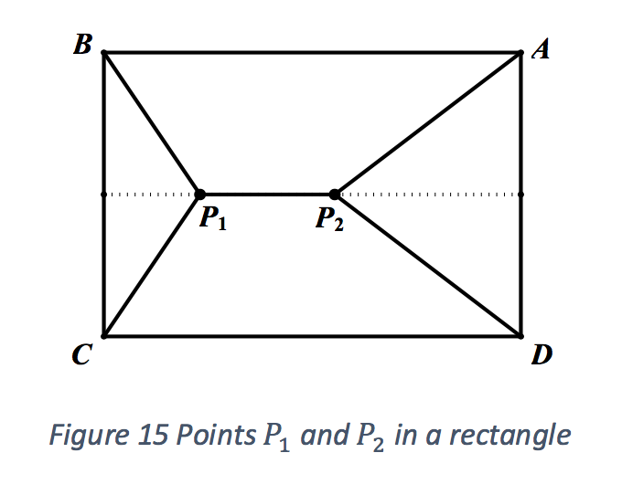
The positions $P_1$ and $P_2$ could bve found with Lemma 1 and Lemma 2 so that $S$ is minimized. Introduction

Without losing generality, assume that in rectangle $ABCD, AB > BC$. For all possible positions of $P_1$ and $P_2$ (figure 16), a point $G$ could always be found on segment $P_1P_2$ so that between $ \bigtriangleup BCP_1$ and $ \bigtriangleup ADP_2$, there is at least one triangle whose three internal angles are less than $120^{\circ}\ $ since $AB > BC$. Introduction

Thus, Fermat point $P_2'$ of $\bigtriangleup AGD$ could be found, obtaining the minimum value of $AP_2' + DP_2' + GP_2'$. And $P_2'$ must be on the straight line $P_1P_2$, as Fermat point of an isosceles triangle must fall on its height on the base (i.e. isosceles triangle $AGD$'s Fermat point $P_2'$ falls on its base $AD$. For new $ P_1P_2$, there must be a point $G$ on it that Fermat point $P_1'$ of $\bigtriangleup BCG$ could be found. And $P_1'$ and $P_2'$ would generate the minimum $S$ for rectangle.

Original Proof of Steiner Point of a Convex Quadrilateral

From Rectangle to Quadrilateral

To further extend the earlier result from rectangles to convex quadrilateral, the rectangle method is applied in a more general case – convex quadrilateral case. However, as quadrilaterals have arbitrary sides and angles, the rectangular strategy is not applicable anymore. Thus, this paper will use the idea of continuous optimization and provide an original proof here, employing various techniques such as recursive algorithms (page 18-20), mathematical induction (page 21), concept of limits and proof by contradiction (page 25-28), which is not in existing literature review.

The overview of the proof is listed below:

1. Reducing all the possible scenarios to the two-point case.

2. Using recursive algorithm and Mathematical Induction to prove that exact Steiner points can be obtained.

3. Using limits, to establish that the two Steiner points found will generate the minimum total distance ($S$).

4. Use proof by contradiction to show that no other more optimal points can be found.

Recursive algorithm for Convex Quadrilaterals

Reducing all the possible scenarios to the two-point case

Lemma 4 For a convex quadrilateral, $S_min$ is obtained when there are two points inside the quadrilateral.

Proof Given only one point inside the convex quadrilateral, the intersection of the two diagonals will be the point that minimizes 𝑆. Introduction

In figure 18 above, applying Triangle Inequality Theorem , $$ AE' + CE' > AC $$ $$ BE' + DE' > BD $$ Thus, $$ BE + AE' + CE' + DE' > BE + AE + CE + DE $$

Enter title here

Hence, for any convex quadrilateral with one point inside, the intersection of twodiagonals will be the point that creates the minimum value for S.

If more than one point are in quadrilateral ABCD (figure19), without losing generality, it can be assumed that ∠BEC < 90° <∠AEB. Since both ∠BEC and ∠AED are smaller than 120°, Fermat points P₂ and P₁ could always be found for both ΔAED and ΔBEC so that

$$BP_1 + CP_1 + P_1E < BE + CE and AP_2 + DP_2 + EP_2 < AE + DE.$$

Notice P₁E and P₂ do not need to be collinear, if not, connecting P₂ do not need to be collinear, if not, connecting P₁ and P₂, P₁E + P₂E > P₁P₂ always holds in ΔP₁EP₂.

For three or more points in the convex quadrilateral (figure 20), one of the points that is extra can always be spotted and the values of S would decrease by eliminating the point(P₂ here). Introduction Hence, for any S of one-point cases and three-or-more-point cases, a smaller value of S will always exist using two points in the given convex quadrilateral.

Original Recursive Algorithm for Convex Quadrilateral cases

Given that only two-point cases are considered, this paper creates an original recursive algorithm to gradually reduce S. For quadrilateral ABCD:

The flowchart of the recursive process is shown below, Introduction

Lemma 5E_n,F_{a_n},F_{b_n} can always be found for all n ∈ $ \mathbb{N}$ and ∠AE_nB ∠CE_nD ≤ 120°

Proof by Mathematical Induction

Proposition:

E_n,F_{a_n},F_{b_n} can always be found for all n ∈ $ \mathbb{N}$ and ∠AE_nB ∠CE_nD ≤ 120°

The Basis:

Given the position of E₀ assuming ∠AE_nB ∠CE_nD ≤ 120° without losing generality, F_a₁,F_b₁ can always be found since ΔAE₀B,ΔCE₀D exist.

The Inductive Step:

Assume E_k exists and ∠AE_kB,∠CE_kD ≤ 120° for some k ∈ $ \mathbb{N}$.

F_{a_k+1},F_{b_k+1} exist and are Fermat points of triangles whose largest angles are no bigger than 120°, so ∠A_{F_{a_k+1}}B, ∠C_{F_{b_k+1}}D = 120°.

For a point E_k+1 on F_{a_k+1'}

∠AE_k+1B ≤ ∠AF_{a_k+1}B = 120°

∠CE_k+1D ≤ ∠CF_{b_k+1}D = 120°

By mathematical induction, E_n F_{a_n} and F_{b_n} could always be found and the lemma is proben.

Lemma 5 proves that Fermat points with angles bigger than 120° are not involved in this algorithm. Thus, all discussions below only concern Fermat points with 120° angles.

The monotonically decreasing sequence from the recursive algorithm

This algorithm creates a monotonically decreasing sequence of the value of S after each manipulation of generating a new pair of Fermat points.

Definition 2 Let F_a₀, F_b₀ be two arbitrary points in a convex quadrilateral ABCD. F_{a_n}, F_{b_n} are the Fermat points of ΔABE_n-1 ΔCDE_n-1 respectively for n ∈ $ \mathbb{N}$ where E_n is a point on F_{a_n}. {S_n} forms a sequence where S_n = AF_{a_n} + BF_{a_n} + CF_{b_n} + DF_{b_n} + F_{a_n}F_{b_n}.

Lemma 6 {S_n} is a monotonically decreasing sequence.

Proof Consider F_{a_n-1},F_{b_n-1} in ABCD below. For any point E_n-1 on F_{a_n-1}F_{b_n-1} such that ∠AE_n-1B, ∠CE_n-1D ≤ 120°, construct ΔABE_n-1 and ΔCDE_n-1. Two Fermat points F_{a_n},F_{b_n} of the two new triangles are found.

To prove that S reduces after each recursion, what is needed to be proven is S_n ≤ S_n-1 holds for all positive integer value of n.

In figure 29, S_n is the sum of lengths of red edges and S_n-1 is the sum of lengths of the green edges.E_n-1 is a random point on F_{a_n-1}F_{b_n-1} and F_{a_n} and F_{b_n} are the Fermat points of ΔABE_n-1 and ΔCDE_n-1 respectively.

By Triangle inequality,

F_{a_n}F_{b_n} ≤ F_{a_n}E_n-1 + F_{b_n}E_n-1

Applying the property of Fermat point of ΔABE_n-1

AF_{a_n} + BF_{a_n} + F_{a_n}E_n-1 < AF_{a_n-1} + BF_{a_n-1} + F_{a_n-1}E_n-1

Applying the property of Fermat point of ΔCDE_n-1

CF_{b_n} + DF_{b_n} + F_{b_n}E_n-1 < CF_{b_n-1} + DF_{b_n-1} + F_{b_n-1}E_n-1

Summing up both sides of the three inequalities above,

F_{a_n}F_{b_n} + AF_{a_n} + BF_{a_n} + F_{a_n}E_n-1 + CF_{b_n} + DF_{b_n} + F_{b_n}E_n-1 < F_{a_n}E_n-1 + F_{b_n}E_n-1 AF_{a_n-1} + BF_{a_n-1} + F_{a_n-1}E_n-1 + CF_{b_n-1} + DF_{b_n-1} + F_{b_n}E_n-1

Since

Thus

holds for all . And the equity is obtained only when the two points and are exactly the same points as and . Thus, is a monotonically decreasing sequence.

Lemma 7 converges to a finite value.

Proof Since and since the sum of lengths of five segments could not be a non-positive value for .

The completeness of real number (Least Upper Bound Property)

Definition 3 Least Upper Bound Property

If represents an ordered set. It will have the least upper bound if, whenever a subset ( is nonempty) is bounded above, then in , has a least upper bound. Then the supremum of , , can denote the least upper bound of . [1]

Theorem 3

If represents an ordered set and it has the least upper bound property. If there is a subset ( is nonempty) that is bounded below, then in , has a greatest lower bound. Then the infimum of , , can denote the greatest lower bound of . [2]

So based on theorem 3, since and , serves as the lower bound for the real set . Therefore, there exists .

Besides, by applying the second lemma of the monotone convergence theorem, which states that

“If a sequence of real numbers is decreasing and bounded below, then its infimum is the limit.” [3]

Since for , the sequence is a decreasing sequence and since it has infimum as proved by the completeness of real number. Thus, by the monotone convergence theorem, .

Theorem 4 .

Proof Let be the set of all possible values of for a quadrilateral as defined above (i.e. the set for all possible values of generated by all possible locations of the two points inside the quadrilateral). Clearly, infinitesimal shifting of the points leads to infinitesimal change in value, so the set will have its upper bound (maximum value) and its lower bound (minimum value) . Therefore, is hence bounded by these two values, .

It is known that since the values of generated from the recursion are only some possible values in all possibilities. Thus, .

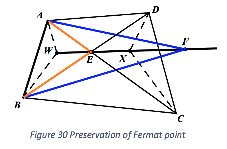
Then the recursive algorithm could be proven to be valid if the value it converges to is the same as the minimum value in all possibilities, which is . This is proved by contradiction in the following session.

if $\lim\limits_{n \to \infty} S_n \neq S_{min}$ $inf\{S_n\} > inf\{S\}$ so $inf\{S_n\} \in \{S\}$. This means a two-point set {W,X} corresponding to $inf\{S_n\}$ can always be found. Let S_min correspond to {Y,Z}. As $inf\{S_n\}$ = $inf\{S_n\} = \lim\limits_{n \to \infty} S_n$, for any point E on ray WX(no matter inside ABCD or outside ABCD), Fermat points of $\bigtriangleup AEB, \bigtriangleup CED$ are still W,X. Otherwise the algorithm produces a smaller S, which contradicts. As Fermat point is the three 120 °, for any point F on line WX but not on the segment (Figure 30), the Fermat point on the other side of the segment still preserves.

Similarly, for S_min Y,Z preseves for triangles formed by any point on YZ and one of them preserves for a point on the line but not segment.

Line WX,YZ cannot be parallel as all angles on each Fermat point must be 120°. Similarly, the four points must be distinct. If they intersect at G, without losing generality, let ΔAGB be the triangle of which the Fermat point preserves. Then each set contributes one Fermat points in ΔAGB that are distinct as in figure 31. Uniqueness of Fermat points leads to contradiction. Thus, $inf\{S_n\}$ = $inf\{S_n\}$ and $\lim\limits_{n \to \infty} S_n = S_{min}$. It is thus proven that the proposed algorithm can find positions of the two Steiner points in a convex quadrilateral.

Python Implementation of Original Recursive Algorithm

With the idea of Finding Fermat points recursively, the following Python implementation provides an algorithm which receives coordinates of four points as input and returns output as coordinates of the two Steiner Points as well as the number of recursive calls made for the purpose of runtime analysis. (Code below generated in planetB) Introduction

Runtime Analysis of Original Recursive Algorithm

Existing algorithms are mainly “brute force” algorithms based on Prim’s algorithm and Kruskal’s algorithm. Undoubtedly, these two algorithms are efficient in finding Minimum Spanning Trees but their runtime complexity in solving STP is still extremely high because the problem involves extra points (Steiner Points) other than existing vertices. This fact makes the STP a NP-Hard problem. However, the recursive algorithm has a much better runtime performance in four-point convex situations.

Raw data of numbers of recursive calls

Rectangle Test

Input coordinates: (0,50), (0,0), (100,0), (100,50)

Output coordinates of Steiner Points: (14.4337,24.9999), (85.5662,24.9999)

Table of Accuracy versus number of recursion counts:

Parallelogram Test

Input coordinates: (-60,0), (-10,-20), (60,0), (10,20)

Output coordinates of Steiner Points: (-12.1254, -12.3527),(12.1254,12.3526)

Table of Accuracy versus number of recursion counts:

Trapezium Test

Input coordinates: (20,50), (0,0), (100,0), (90,50)

Output coordinates of Steiner Points: (25.4496,39.3555), (36.5372)

Table of Accuracy versus number of recursion counts:

Random Convex Quadrilateral Test

Input coordinates: A(20,60), B(-80,20), C(0,-60), D(100, 30)

Output coordinates of Steiner Points: (11.4814,36.3966),(27.8023,17.0601)

Introduction

Table of Accuracy versus number of recursion counts:

Approximation Algorithm Analysis

Due to the constrains of computer (its smallest division limit), the test continues up to a certain level of accuracy (mostly up to ±10^-15). However, these data are sufficient to justify the runtime complexity of the recursive algorithm. It is very difficult to give the overall runtime of recursive algorithm in "Big O" or "Big 0" notation because the input is always the coordinates of the four points, and quantifying the "complexity" of a geometric shape is extremely difficult. Besides, as a recursive algorithm, it will not computationally reach the exact solution using computer (although the theoretical correctness of this algorithm is proven mathematically in previous section). However, the relationship between the accuracy and the number of recursive calls exhibits a very convincing pattern that this recursive algorithms performs much better than any other algorithms using "brute force". The relationship between the improvement on accuracy (adopts 1/Accuracy for convenience) and the number of recursive calls of the previous four tests is presented below.

Approximation Algorithm Analysis

Due to the constrains of computer (its smallest division limit), the test continues up to a certain level of accuracy (mostly up to $\pm$ $10^{-15}$). However, these data are sufficient to justify the runtime complexity of the recursive algorithm. It is very difficult to give the overall runtime of recursive algorithm in "Big O" or "Big $\theta$" notation because the input is always the coordinates of the four points, and quantifying the "complexity" of a geometry shape is extremely difficult. Besides, as a recursive algorithm, it will not reach the exact solution using computer (although it will definitely be proven by mathematics in previous sections). However, the relationship between the accuracy and the number of recursive calls exhibits a very convincing pattern that this recursive algorithms performs much better than any other algorithms using "brute force". The relationship between the improvement on accuracy (adopts 1/Accuracy for convenience) and the number of recursive calls of the previous four tests is presented below.

Rectangle and Parallelogram cases $\Longrightarrow$ $\theta(1)$

For both rectangle and parallelogram cases, the algorithm terminates after its first call, meaning that only one recursive call is needed to find the most optimal solution for all rectangles and parallelogram cases. Therefore, the runtime complexity is $\theta(1)$.

Trapezium case

For a trapezium test, the recursive algorithm takes only 9 calls to reach the $\pm$ 0.1 accuracy, which indicates that the recursive algorithm is also very efficient in reaching an solution that is relatively accurate. Furthermore, as the accuracy improves 10 times, the number of recursive calls only increases linearly . This implies that as accuracy increases exponentially, the runtime complexity increases only linearly, which is much more efficient than existing STP algorithms. Note: for visualization purpose, runtime growth = number of recursive calls x $10^{11}$

Random Convex Quadrilateral case

Test results for random convex quadrilateral is very similar to the case of trapezium. The data also show that the recursive algorithm converges very fast. The difference in the slope of Line Of Best Fit is most likely due to the randomness of the shape. Note: for visualization purpose, runtime growth = number of recursive calls x $10^{12}$

Application

Now the real-life problem mentioned in introduction could be completely solved using the recursive algorithm proven in previous section.

By applying the recursive algorithm, the intersection of two diagonals, $E_0$ could be found.

Then, the recursive algorithm could be applied and infinite pairs of Fermat points could be determined and the two points after first manipulation are found as SD and SE in figure 37. In real-life application, it is not necessary for the construction company to determine the exact Steiner points since $1^{\circ}$ will not cause a huge increase in total distance. Thus, it could be assumed that the optimal situation is achieved if the six angles around two junctions are $120^{\circ} \pm 1^{\circ}$.

The construction of Fermat point in figure 38 is referenced from C. Kimberling.

From the measurement in figure 3918, all six angles are within the range of $120^{\circ}$ $\pm$ $1^{\circ}$, the assumed optimal case is achieved after one manipulation and the actual construction suggestion is shown below.

Since $\textit{MN}$ is 50 km, the five roads needed to be built are shown in blue in figure 41,

Conclusion

Finding the minimal distance to connect multiple points has numerous applications. This problem is related to the Steiner Tree Problem and modelled using graph theory. Generally, the solution would involve finding a point set within the convex hull of the given set of vertices, and connect the vertices to the closest points in the point set and between the points in that point set. For triangle case, the solution is to connect the Fermat point to three vertices. The case of quadrilateral is the focus of this project. The rectangle case is first investigated. It is proven that when the optimal connection is made, there are two points within the rectangle. The positions of the two points are then proven to be on the longer segment of symmetry of the rectangle. It is then proven that the three angles on each of the two points within the rectangle must be $120^{\circ}$. This enables us to find the two-point point set given any rectangle. For an arbitrary convex quadrilateral, the two-point criterion is proven too. An original recursive algorithm is proposed to create a sequence of two-point point sets. The existence of such point set in each step of the algorithm is proven inductively, and the sequence of the total distance is proven to be monotonically decreasing and converges to the minimal possible total distance. Finally, the python implementation provides an exact algorithm that could directly solve all four-point problems. Further analysis over runtime complexity assures that the original recursive algorithm has much better performance than existing algorithms: as accuracy improves exponentially, there is only a linear increase in runtime for this recursive algorithm.

Bibliography

[1] M. Brazil, R. L. Graham, D. A. Thomas and M. Zachariasen, "On the History of the Euclidean Steiner Tree Problem".
[2] C. Donghui, D. D. Zhu, H. X. Dong, G. H. Lin, L. Wang and G. Xue, "Approximations for Steiner tree with minimum number of Steiner points," Theoretical Computer Science, vol. 262, pp. 83-99, 23 March 2000.
[3] G. Soothill, "The Euclidean Steiner Problem," Durham, 2010.
[4] F. Hwang, D. Richards and P.Winter, The Steiner Tree Problem, Elsevier Science Publishers, 1992, pp. 1-353.
[5] Hajia and Mowaffaq, "An Advanced Calculus Approach to Finding the Fermat Point," Mathematics Magazine, p. 29.
[6] E. Abbena, S. Salamon and A. Gray, Modern Differential Geometry of Curves and Surfaces with Mathematica, Chapman and Hall/CRC; 3 edition, 2006, p. 1016.
[7] T. H. Cormen, Introduction to Algorithms, Illustrated ed., MIT Press, 2009, pp. 634-651.
[8] K. M. Koh, F. M. Dong and E. G. Tay, Introduction to Graph Theory: H3 Mathematics, Illustrated ed., World Scientific, 2007, pp. 1-15.
[9] R. Diestel, "Graph Theory," in Graduate Texts in Mathematics, 3rd ed., vol. 173, Springer-Verlag, 2005, pp. 6-9.
[10] "The Fermat Point and Generalizations," Spot. IM Ltd., 17 October 2015. [Online]. Available: http://www.cut-the-knot.org/Generalization/fermat_point.shtml#. [Accessed 6 March 2016].
[11] M. Hazewinkel, Ed., The Encyclopedia of Mathematics, Springer, 2001.
[12] "WolframMathWorld," Mathematica Technology, 1999-2006. [Online]. Available: http://mathworld.wolfram.com/GraphCycle.html. [Accessed 6 March 2016].
[13] R. N. Aufmann and R. D. Nation, Algebra and Trigonometry, 8, illustrated ed., Cengage Learning, 2014, pp. 601-603.
[14] J. Herman, R. Kucera and J. Simsa, Equations and Inequalities: Elementary Problems and Theorems in Algebra and Number Theory, illustrated ed., Springer Science & Business Media, 2012, pp. 151- 153.
[15] W. C. Bauldry, Introduction to Real Analysis: An Educational Approach, John Wiley & Sons, 2011, pp. 47-48.
[16] J. Yeh, Real Analysis: Theory of Measure and Integration, World Scientific, 2006, pp. 14-17.
[17] C. Kimberling, Geometry in Action: A Discovery Approach Using the Geometer's Sketchpad, illustrated ed., Springer Science & Business Media, 2003, p. 15.
[18] J. Weng, "Variational approach and Steiner minimal trees on four points," Discrete Mathematics, vol. 132, no. 1-3, pp. 349-362, 11 November 1992.
Unless mentioned, all figures in this paper were drawn using Geometer’s Sketchpad.

Appendices

Proof of Fermat point of a triangle is the Steiner point in triangle cases

In $\Delta$ABC below, $\textit{P}$ is a random given point in the triangle. If there are more than one point in the triangle and $\textit{S}$ is minimized, the point $\textit{P'}$ is taken as the second point.

Thus, $\textit{S}$ would be reduced if paths $\textit{PP'}$ and $\textit{P'C}$ are replaced by $\textit{PC}$. Therefore, given point $\textit{P}$, any additional point other than $\textit{P} would increase the value of $\textit{S}$ since there will always be a case of one point which achieves a smaller $\textit{S}$ compared to multiple points.

Theorem 1

$\textit{In any given triangle ABC, S is minimized when the point inside triangle is its Fermat point.}$

Proof

If an arbitrary triangle $\textit{ABC}$ as the figure shown, as what is proved in the earlier section, the Steiner point of any triangle should be found inside the triangle. Establishing a coordinate system, take $\textit{P}$ as a random point with coordinates $\textit{(x, y)}$ while points $\textit{A}$, $\textit{B}$, and $\textit{C}$ have their coordinates $(x_{A},y_{A}),(x_{B},y_{B},(x_{C},y_{C})$ .

After substituting in the coordinates of segments $\textit{PA}$, $\textit{PB}$ and $\textit{PC}$, the expression for $\textit{s}$ could be obtained as followed via the Pythagoras Theorem, $$S = \sqrt{(x - x_{A})^2 + (y - y_{A})^2} + \sqrt{(x - x_{B})^2 + (y - y_{B})^2} + \sqrt{(x - x_{C})^2 + (y - y_{C})^2} $$ By taking its partial derivatives with regard to $\textit{x}$ and $\textit{y}$, and take their minimum value, $$\frac{\delta S}{\delta x} = \frac{x - x_{A}}{\sqrt{(x - x_{A})^2 + (y - y_{A})^2}} + \frac{x - x_{B}}{\sqrt{(x - x_{B})^2 + (y - y_{B})^2}} + \frac{x - x_{C}}{\sqrt{(x - x_{C})^2 + (y - y_{C})^2}} = 0$$ $$\frac{\delta S}{\delta x} = \frac{y - y_{A}}{\sqrt{(x - x_{A})^2 + (y - y_{A})^2}} + \frac{y - y_{B}}{\sqrt{(x - x_{B})^2 + (y - y_{B})^2}} + \frac{y - y_{C}}{\sqrt{(x - x_{C})^2 + (y - y_{C})^2}} = 0$$ pg47
According to the figure, $$\frac{x - x_{A}}{PA} + \frac{x - x_{B}}{PB} + \frac{x - x_{c}} = 0$$ $$\frac{y - y_{A}}{PA} + \frac{y - y_{B}}{PB} + \frac{y - y_{c}} = 0$$ Transfer these two equations to dot product in vector forms,
Since $$ \alpha \cdot \delta = \beta \cdot \delta = 0 $$
Hence $\delta$ is perpendicular to both $\alpha$ and $\beta$, and thus parallel to the cross product between $\alpha$ and $\beta$, $$ \begin{align*} \alpha \times \beta = \begin{pmatrix} x - x_A\\ x - x_B\\ x - x_C \end{pmatrix} \times \begin{pmatrix} y - y_A\\ y - y_B\\ y - y_C \end{pmatrix} \\ = \begin{pmatrix} \begin{vmatrix} x - x_B & y - y_B \\ x - x_C & y - y_C \end{vmatrix} \\ - \begin{vmatrix} x - x_A & y - y_A \\ x - x_C & y - y_C \end{vmatrix} \\ \begin{vmatrix} x - x_A & y - y_A \\ x - x_B & y - y_B \end{vmatrix} \end{pmatrix} \\ \end{align*} $$
Thus, as shown in Figure 46, pg47
$$ \begin{vmatrix} x - x_{A} & y - y_{A} \\ x - x_{C} & y - y_{C} \end{vmatrix} = (x - x_{A})(y - y_{C}) - (x - x_{C})(y - y_{A}) = -2 \times \text{Area of} \bigtriangleup APC $$
Similarly, $$ \begin{vmatrix} x - x_{A} & y - y_{A} \\ x - x_{C} & y - y_{C} \end{vmatrix} = (x - x_{A})(y - y_{C}) - (x - x_{C})(y - y_{B}) $$
Thus, $$ (x - x_{A})(y - y_{C}) - (x - x_{C})(y - y_{B}) = AF \times GH + EF \times DE $$
Besides, pg47
$$ Area of \bigtriangleup APC = \frac{1}{2} AE \times AH - GP \times GH - \frac{1}{2} (AF \times AG) - \frac{1}{2}(PD \times PI) $$
$$ Area of \bigtriangleup APC= \frac{1}{2} AE \times AH - GP \times GH - \frac{1}{2} (AF \times AG) - \frac{1}{2}(PD \times PI) $$ $$ \begin{align*} 2 \times Area of \bigtriangleup APC = (AF + EF)(AG + GH) - 2 \times GP \times GH - (AF \times AG) - (EF \times DC) \\ = AF \times GH + EF \times AG - 2 \times AF \times GH \\ = EF \times AG - AF \times GH \\ = (x_{c} - x)(y_{A} - y) - (x - x_{A})(y - y_{C}) \end{align*} $$ $$ \begin{vmatrix} x - x_{A} & y - y_{A} \\ x - x_{C} & y - y_{C} \end{vmatrix} = (x - x_{A})(y - y_{C}) - (x - x_{C})(y - y_{A}) = -2 \times \text{Area of} \bigtriangleup APC $$
For the same reason and method, $$ \begin{vmatrix} x - x_{A} & y - y_{A} \\ x - x_{B} & y - y_{B} \end{vmatrix} = (x - x_{A})(y - y_{B}) - (y - y_{A})(x - x_{B}) = -2 \times \text{Area of} \bigtriangleup PAB $$
Therefore, convert the previous cross product to the following expression,
$$ \begin{align*} \alpha \times \beta = \begin{pmatrix} x - x_A\\ x - x_B\\ x - x_C \end{pmatrix} \times \begin{pmatrix} y - y_A\\ y - y_B\\ y - y_C \end{pmatrix} \\ = \begin{pmatrix} \begin{vmatrix} x - x_B & y - y_B \\ x - x_C & y - y_C \end{vmatrix} \\ - \begin{vmatrix} x - x_A & y - y_A \\ x - x_C & y - y_C \end{vmatrix} \\ \begin{vmatrix} x - x_A & y - y_A \\ x - x_B & y - y_B \end{vmatrix} \end{pmatrix} \\ = \begin{pmatrix} \mp 2 \times \text{Area of} \bigtriangleup PBC\\ \mp 2 \times \text{Area of} \bigtriangleup PAC\\ \mp 2 \times \text{Area of} \bigtriangleup PAB\\ \end{pmatrix} \end{align*} $$
Since $$ 2 \times \text{Area of} \bigtriangleup PBC = 2 \times \frac{1}{2} \times |\overrightarrow{PB}| \times |\overrightarrow{PC}| \times sin \angle BPC $$ $$ 2 \times \text{Area of} \bigtriangleup PAC = 2 \times \frac{1}{2} \times |\overrightarrow{PA}| \times |\overrightarrow{PC}| \times sin \angle APC $$ $$ 2 \times \text{Area of} \bigtriangleup PAB = 2 \times \frac{1}{2} \times |\overrightarrow{PB}| \times |\overrightarrow{PA}| \times sin \angle BPA $$
Thus, $$ \alpha \times \beta = \begin{pmatrix} \mp |\overrightarrow{PB}| \times |\overrightarrow{PC}| \times sin \angle BPC\\ \mp |\overrightarrow{PA}| \times |\overrightarrow{PC}| \times sin \angle APC\\ \mp |\overrightarrow{PB}| \times |\overrightarrow{PA}| \times sin \angle BPA \end{pmatrix} $$
Since $\delta$ is is parallel to $\alpha\times\beta$, so for a certain value of $\gamma$, there will be $$ \delta = \begin{pmatrix} \frac{1}{|\overrightarrow{PA}|}\\ \frac{1}{|\overrightarrow{PB}|}\\ \frac{1}{|\overrightarrow{PC}|} \end{pmatrix} = \gamma \begin{pmatrix} |\overrightarrow{PB}| \times |\overrightarrow{PC}| \times sin \angle BPC\\ |\overrightarrow{PA}| \times |\overrightarrow{PC}| \times sin \angle APC\\ |\overrightarrow{PB}| \times |\overrightarrow{PA}| \times sin \angle BPA \end{pmatrix} $$
which is equivalent to $$ \frac{1}{|\overrightarrow{PA}|} = \gamma \times |\overrightarrow{PB}| \times |\overrightarrow{PC}| \times sin \angle BPC $$ $$ \frac{1}{|\overrightarrow{PB}|} = \gamma \times |\overrightarrow{PA}| \times |\overrightarrow{PC}| \times sin \angle APC $$ $$ \frac{1}{|\overrightarrow{PC}|} = \gamma \times |\overrightarrow{PB}| \times |\overrightarrow{PA}| \times sin \angle BPA $$
Hence, as shown in figure 48, with $\gamma$ is a constant value, pg47 $$ \frac{1}{\gamma \times |\overrightarrow{PA}| \times |\overrightarrow{PB}| \times |\overrightarrow{PC}|} = sin \angle BPC = sin \angle APC = sin \angle BPA $$
Since $$ \angle BPC < 180^{\circ} $$ $$ \angle APC < 180^{\circ} $$ $$ \angle BPA < 180^{\circ} $$ And at point $\textit{P}$, $$ \angle BPC = \angle APC = \angle BPA = 360^{\circ} $$
Therefore, $$ \angle BPC = \angle APC = \angle BPA = 120^{\circ} $$

Semester

Spring 2018

Researcher

Ziming Xue and Rigel

Navigation

Abstract
Introduction
Research Question
Literature Review
Mathematical Modelling via Graph Theory
Steiner Point of a Triangle
Original Proof for Steiner Points of a Rectangle
Original Proof of Steiner Point of a Convex Quadrilateral
Approximation Algorithm Analysis
Rectangle and Parallelogram cases
Trapezium case
Random Convex Quadrilateral case
Application
Conclusion
Biblography
Appendices

Executive / Directors

Member Profiles

Internal Affairs

Steiner Tree Problem in Convex Quadrilaterals using Recursive Algorithm

Abstract

Introduction

Research Question

Literature Review

Mathematical Modelling via Graph Theory

Steiner Point of a Triangle

Original Proof for Steiner Points of a Rectangle

Original Proof of Steiner Point of a Convex Quadrilateral

From Rectangle to Quadrilateral

Recursive algorithm for Convex Quadrilaterals

Original Recursive Algorithm for Convex Quadrilateral cases

Proof by Mathematical Induction

The monotonically decreasing sequence from the recursive algorithm

The completeness of real number (Least Upper Bound Property)

Definition 3 Least Upper Bound Property

Theorem 3

Python Implementation of Original Recursive Algorithm

Runtime Analysis of Original Recursive Algorithm

Raw data of numbers of recursive calls

Rectangle Test

Parallelogram Test

Trapezium Test

Random Convex Quadrilateral Test

Approximation Algorithm Analysis

Approximation Algorithm Analysis

Rectangle and Parallelogram cases $\Longrightarrow$ $\theta(1)$

Trapezium case

Random Convex Quadrilateral case

Application

Conclusion

Bibliography

Appendices

Proof of Fermat point of a triangle is the Steiner point in triangle cases

Theorem 1

Proof

Semester

Researcher